Clean controls in practice: estimating debt effects with LP-DiD
LP-DiD, local projections, difference-in-differences, clean controls, TWFE, fiscal policy econometrics
Event studies on macro panels have a quiet problem. In a standard two-way fixed effects setup, countries that treated earlier serve as controls for countries that treat later, and vice versa. When treatment effects are heterogeneous or dynamic, those comparisons contaminate the estimates, a point the difference-in-differences literature has made forcefully over the last few years. Fiscal policy applications are especially exposed, because consolidation episodes cluster in time, think 2010 to 2013, and their effects build slowly.
The Local Projections Difference-in-Differences estimator of Dube, Girardi, Jordà and Taylor (2025, Journal of Applied Econometrics) addresses this with two design choices that are easy to state and easy to audit. In a recent working paper with Cristina Mazas Pérez-Oleaga and José M. Domínguez Martínez, we apply it to 126 fiscal consolidation episodes in the EU-27. A few practical lessons follow.
The two design choices
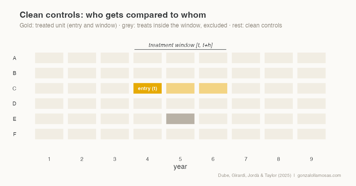
First, treatment is defined as entry. The treatment indicator switches on in the year a country crosses the consolidation threshold, an improvement of at least one percentage point of potential GDP in the structural primary balance, and what is estimated is the effect of entering an episode, horizon by horizon.
Second, and this is the core of the method, the control group at each horizon contains only clean observations, meaning countries that are not treated anywhere in the window from the entry year to the horizon of interest. No forbidden comparisons enter the estimate. The outcome is a long difference from the pre-treatment year, and the specification adds country fixed effects, year-by-horizon fixed effects, two lags of the outcome change and lagged macro controls.
The cost is transparency about sample loss. Of 135 episodes in our panel, 126 survive the clean-control requirement at the impact horizon, and the effective sample shrinks as the horizon lengthens. We report the counts at every horizon, and we would encourage anyone using the method to do the same, because the estimand quietly changes with the surviving sample.
The estimator in a few lines of R
Stripped to its essentials, the whole procedure fits on one screen. For each horizon, build the long difference, flag the units that stay untreated through the window, keep entries and clean controls only, and run the fixed-effects regression.
library(dplyr)
library(fixest)

lpdid_h <- function(panel, h) {
  df <- panel |>
    group_by(country) |>
    mutate(
      d_y   = lead(debt_gdp, h) - lag(debt_gdp, 1),           # long difference
      clean = slider::slide_dbl(entry, max, .after = h) == 0  # untreated in [t, t+h]
    ) |>
    ungroup() |>
    filter(entry == 1 | clean)                                # no forbidden comparisons

  feols(d_y ~ entry + d_debt_l1 + d_debt_l2 + x_l1 | country + year,
        data = df, cluster = ~country)
}

irf <- lapply(0:5, function(h) lpdid_h(panel, h))

# 27 clusters: complement with a wild cluster bootstrap (Webb weights)
fwildclusterboot::boottest(irf[[1]], param = "entry",
                           B = 999, type = "webb")
Each element of irf is one point of the impulse response, and the header figure of this post was drawn with the same logic. The real code adds the placebo horizons, the trimming and the robustness battery, but nothing conceptually new.
What we learned applying it
Inference with 27 clusters deserves more care than the default. We cluster at the country level and complement the usual standard errors with a wild cluster bootstrap using six-point Webb weights, which behaves better with few clusters. Conclusions that survive both are worth keeping; one of our headline results, the short-run increase in the debt ratio, does.
Pre-trends are testable and worth showing in three flavours. We report placebo coefficients at one, two and three years before entry for the baseline specification, for a conditional parallel-trends version and for a propensity-score trimmed sample restricted to common support. All three come out flat, which is what gives the post-treatment estimates their credibility.
Power, not bias, is the binding constraint at long horizons. Our point estimates grow with the horizon while their precision falls, and the honest reading is that the short-run effects are the reliable evidence. Writing that sentence in the paper, rather than hoping a referee will not notice, turned out to be the better strategy.
The full paper, including the debt decomposition that explains why consolidations fail to reduce the ratio, is on ResearchGate and summarised on the Research page.